On this page
Short free text arrives as rows: support reports, app-store reviews, feedback boxes, a comment field nobody designed. The obvious pipeline sends each row to a model and stores the label it returns. The cost is the visible problem. Thousands of rows say “charged twice” in a dozen spellings, and each one is a paid call.
The quieter failure is worse. The same meaning gets labelled several times, and the labels do not have to agree. And once you switch to embeddings to save money, a similarity threshold starts filing a complaint nobody has seen before under the nearest category it already knows, with a score that looks confident.
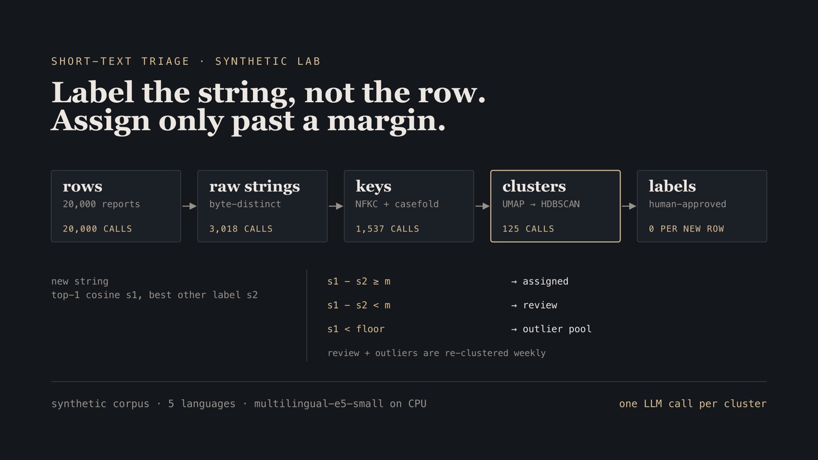
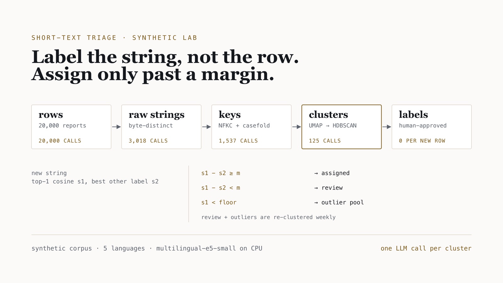
Operating rule. Normalize to a key, embed each distinct key once, cluster the keys, and label the clusters. Then assign a new string only when its best label beats the runner-up by a margin. Strings that fail the margin go to a review queue that is itself clustered. A model never sees a row.
I rebuilt this design as a lab so every number below is reproducible. The design is one I worked on for a client; the client’s data and code stay private, and the corpus here is synthetic.
The rig
Everything is synthetic and seeded. I wrote 240 base phrasings by hand: eight intents a consumer app’s support inbox would see (double charge, missing refund, login failure, app crash, late delivery, account takeover, unwanted marketing, cancellation), in English, Spanish, German, French and Portuguese, six wordings each. A generator damages them the way free-text fields get damaged, then samples them so a few wordings dominate, as they do in real inboxes.
| Corpus | Day 1 | Day 2 |
|---|---|---|
| Rows | 20,000 | 20,000 |
| Day-1 wordings (four of six per intent and language) | 19,394 | 14,086 |
| Wordings held back from day 1 | — | 3,937 |
A ninth intent with no day-1 rows (change_address) |
— | 1,363 |
Content-free noise (ok, test, ?) |
606 | 614 |
The damage mix on day 1 was 9,633 exact copies, 3,039 case changes, 2,426 single-character typos, 2,384 trailing punctuation, 1,640 stray or non-breaking spaces, and 878 accented strings in decomposed Unicode (NFD), as some keyboards and copy-paste paths emit. Day 2 is the test: known wordings with new damage, wordings the system has never embedded, and a category that has no cluster at all.
The model is intfloat/multilingual-e5-small (384 dimensions) on CPU with four threads, on an Apple M5. The machine was shared with other work during the runs, with a load average between 34 and 56. Wall-clock times are inflated, so I report process CPU time as the comparable figure, each the median of three runs. Every number here is in the lab’s MEASUREMENTS.md, with the JSON it came from, and the whole lab is public as short-text-triage.
Rows are the wrong unit of work
The first decision is the cache key. I measured five, each adding one step:
import re, unicodedata

_EDGE = re.compile(r"^[^\w]+|[^\w]+$")

def key(s: str) -> str:
    s = " ".join(s.split())                 # also splits on U+00A0
    s = unicodedata.normalize("NFKC", s)    # precomposes NFD accents
    s = s.casefold()                        # not lower(): ß -> ss
    return _EDGE.sub("", s).strip()         # inner apostrophes survive
| Key | Distinct day-1 keys | Rows per key | Day-2 rows served from cache |
|---|---|---|---|
| Raw bytes | 3,018 | 6.6 | 67.8% |
| + whitespace | 2,624 | 7.6 | 68.5% |
| + NFKC | 2,569 | 7.8 | 68.5% |
| + casefold | 2,182 | 9.2 | 69.0% |
| + edge punctuation | 1,537 | 13.0 | 70.1% |
The full key leaves 49% fewer strings to embed and label than raw bytes. Embedding cost follows the key count almost exactly: 1,537 keys took 6.74 CPU-seconds, and the 20,000 rows took 93.31, a ratio of 13.8 for 13.0 rows per key.
The cache hit rate barely moves, and that needs explaining rather than hiding. Day-1 wordings are 70.4% of day-2 rows, so 70.1% is close to the ceiling. And after 20,000 rows a raw cache has also seen most variants of the popular wordings. Normalization does not mainly buy hit rate in steady state. It buys one label per meaning: with raw keys, Charged twice!!, charged twice and CHARGED TWICE are three cache entries, three paid labels, and three chances to disagree.
What normalization collapses, and what it cannot
Of the 1,537 keys, 1,364 (88.7%) first appeared as a typo. The other 173 are exactly the 160 day-1 wordings plus 13 noise keys. The key function folded every mechanical variant back onto its base wording, and nothing else. What stays distinct after normalization is misspelling, and only the embedding step can fold that.
Two smaller findings belong in any implementation. ? and ... both normalize to the empty string, which will happily get a label unless the pipeline drops empty keys first. And lower() is the wrong call: "Straße".lower() stays straße, while casefold() gives strasse.
The NFD miss only shows up when a source changes
The textbook argument for NFKC is that débité typed on one device and pasted from another are different byte strings. In steady state the lab barely shows it: of 613 day-2 rows in decomposed form whose wording existed on day 1, a raw-key cache missed 8, because day 1 had already seen decomposed copies of the popular wordings.
Then I ran the scenario that actually happens. The cache is filled from sources that only ever sent composed text, and one source starts sending NFD. A new app version or keyboard is enough. The raw-key cache missed 613 of 613. The normalized key missed none. Nothing errors when this happens. The cache stops hitting for one cohort, the bill rises, and labels drift. NFKC is cheap insurance against a change you will not be told about.
Cluster distinct keys, not rows
I clustered day 1 three ways and scored the result against the planted intents, weighted by rows:
| Method | Points | CPU s | Clusters | Noise rows | Purity | Multilingual clusters |
|---|---|---|---|---|---|---|
| HDBSCAN on 384-d vectors, distinct keys | 1,537 | 1.22 | 97 | 4.9% | 99.6% | 19.6% |
| UMAP → HDBSCAN, distinct keys | 1,537 | 3.30 | 124 | 2.1% | 99.5% | 25.8% |
| UMAP → HDBSCAN, every row | 20,000 | 35.44 | 1,254 | 11.9% | 99.98% | 1.0% |
The row-level run is the instructive failure. Its purity is nearly perfect, and it is still useless. A popular string repeated five times satisfies min_cluster_size=5 all by itself, so density clustering turns into a frequency counter. Each popular spelling becomes its own cluster, and cross-language grouping collapses to 1%. Labelling that output costs 1,254 calls instead of 124, after ten times the clustering CPU.
The received wisdom did not survive contact with this corpus either. “Always reduce with UMAP before HDBSCAN” holds for large, high-dimensional sets. On 1,537 points, plain HDBSCAN on the raw vectors was just as pure. UMAP’s contribution was a lower noise share and more clusters that span languages. I kept UMAP for that reason, not because the 384-d run failed.
Both distinct-key runs split each intent into 9 to 21 fine clusters, usually one wording family per cluster. That is the intended output. Fine clusters become subcategories; one extra call over the cluster labels proposes the broad categories; a person approves both. Day 1 cost 124 cluster calls plus that one, 125 in total, against 20,000 per row.
On short text, cosine lives in a band
The next decision is how a new string joins an existing cluster, and it depends on what the similarity scores look like. I measured every pair of the 240 clean wordings (28,680 pairs) with the query: prefix:
| Pairs | p5 | p50 | p95 |
|---|---|---|---|
| Same intent | 0.802 | 0.854 | 0.926 |
| Different intent | 0.776 | 0.819 | 0.866 |
| All | 0.777 | 0.822 | 0.879 |
The lowest score among all 28,680 pairs was 0.715. 76% of different-intent pairs scored above 0.80, and 45% of same-intent pairs scored below 0.85. The two distributions overlap across most of their range, and that is the geometry of short text in this model: everything is fairly similar to everything. A threshold of 0.85 does not separate “same meaning” from “different meaning”; as the next section shows, it rewards shared vocabulary at least as much as shared intent.
The prefix did not matter. Consistency still does.
The e5 model card asks for a query: or passage: prefix, and I expected leaving it off to cost precision. It did not, measurably. Nearest-neighbour precision on the 240 wordings was 0.933 with query: , 0.896 with passage: , and 0.963 with no prefix. Cross-lingual precision was 0.975, 0.992 and 0.971. Mixing prefixes between index and probe stayed in the same range.
What the prefix does change is position. The same text embedded with query: and with passage: has a mean cosine of 0.943 to itself, a shift of 0.057. The next section rests on a decision margin of 0.03. A cache embedded one way and new strings embedded another would put the same text 0.057 away from itself on average, nearly twice the margin, and nothing would raise an error. Pin the prefix with the model revision, version both, and re-embed when either changes.
A threshold is not a decision. A margin is.
On day 2, 13,718 rows hit the label cache at 99.5% label precision. The remaining 6,282 rows over 1,243 keys had to be placed against the day-1 cluster centroids. Before any policy, the nearest centroid alone was right for 97.2% of typos of known wordings, 55.0% of wordings it had never seen, and 0% of the unseen category, which has no centroid to be right about.
That 55% is the real problem, and one string shows it. je n'arrive pas à me connecter à mon compte (“I can’t connect to my account”) is a login failure, 830 rows of it. Its nearest centroid is the account-takeover cluster built around quelqu'un s'est connecté à mon compte (“someone connected to my account”), at 0.953. Same words, opposite meaning, and a score higher than most correct matches.
An absolute threshold cannot handle that:
| Absolute τ | Assigned rows | Precision | Unseen-category rows assigned |
|---|---|---|---|
| 0.85 | 6,253 | 50.0% | 1,358 of 1,363 |
| 0.90 | 4,424 | 57.8% | 165 |
| 0.92 | 2,862 | 66.2% | 0 |
| 0.94 | 1,982 | 54.2% | 0 |
Raising the threshold to 0.94 made precision worse, because the most confident wrong answer clears every threshold, and at 0.94 it is 830 of the 1,982 rows assigned. The unseen category sat between 0.861 and 0.911 (p5–p95), inside the range where correct matches live, so it was only excluded once the threshold also discarded most good matches.
The margin asks a different question: does the best label beat the best different label by enough?
def decide(sims, labels, floor=0.80, m=0.03):
    top = sims.argmax()
    s1, label = sims[top], labels[top]
    s2 = sims[labels != label].max()        # best competing label, not 2nd centroid
    if s1 < floor:
        return "outlier", label, s1
    if s1 - s2 >= m:
        return "assigned", label, s1
    return "review", label, s1
| Margin m | Assigned rows | Precision | Unseen-category rows assigned | Sent to review |
|---|---|---|---|---|
| 0.01 | 4,770 | 60.1% | 498 | 1,512 |
| 0.02 | 2,994 | 63.4% | 162 | 3,288 |
| 0.03 | 1,728 | 95.2% | 48 | 4,554 |
| 0.04 | 1,354 | 95.9% | 46 | 4,928 |
| 0.08 | 399 | 100% | 0 | 5,883 |
At m = 0.03, precision on assigned rows is 95.2% against 66.2% for the best absolute threshold, while assigning fewer rows (1,728 against 2,862) and sending the rest to a queue rather than to a wrong label. 1,315 of the 1,363 unseen-category rows went to review instead of an existing label. Correct top-1 matches had a median margin of 0.065; wrong ones 0.010.
One caveat changes how you set m. The jump from 63% to 95% between 0.02 and 0.03 is mostly that single French string, whose margin is 0.0298. On a Zipf-shaped corpus one heavy string can move row-weighted precision by thirty points. Pick m from a labelled sample of your own traffic, weighted by row, and look at the heaviest strings on both sides of the line before trusting the curve. The floor caught nothing here, because every cache miss scored at least 0.80. It belongs in the policy for content-free input, but the margin did the work.
The review pool is where the new category shows up
Sending 4,554 rows to review sounds like a staffing problem. It is not, because review is clustered too. The 515 refused keys went through the same UMAP → HDBSCAN step and became 44 clusters. Fourteen were majority change_address. They held 1,298 of the 1,315 unseen-category rows that reached the pool, at 97.2% purity. A reviewer reads 44 groups, approves one new category with a few subcategories, and folds the stray French login wording back into login failure.
| Unit of work | Day 1 calls | Day 2 calls |
|---|---|---|
| Per row | 20,000 | 20,000 |
| Per distinct normalized key | 1,537 | 1,243 |
| Per cluster | 125 | 44 |
Assigned rows cost nothing on day 2. The calls go to the clusters a person has to look at anyway.
Boundary. The corpus is synthetic: 240 hand-written wordings in five Latin-script languages, damaged by a seeded generator. Real traffic has longer tails, mixed scripts, sarcasm and code-switching, so the cluster counts and precision figures will move. What should transfer is the shape: per-row and per-key costs differ by the rows-per-key ratio; exact duplicates break density clustering; short-text cosine scores crowd into a narrow band; and a margin outperforms an absolute threshold when lexical overlap and meaning disagree. Two claims I expected to confirm did not reproduce here: UMAP was not needed for purity at this size, and omitting the e5 prefix did not hurt precision. Timings come from one shared machine under load; compare CPU seconds, not wall-clock. No LLM was called; call counts are what each unit of work would cost.
What I would carry into a production pipeline
- One key function, versioned, applied on write and on lookup: whitespace, NFKC, casefold, edge punctuation, then drop empty keys.
- Label cache keyed on that key, carrying the model revision, prefix, taxonomy version and label source.
- Embed distinct keys only, with the prefix pinned alongside the model revision; re-embed when either changes.
- Cluster distinct keys, never rows; carry row counts as weights, not as duplicate points.
- One call per cluster to propose labels, one call to group them into categories, then a person approves.
- Assign with a margin against the best different label, set from a labelled, row-weighted sample.
- Cluster the review and outlier pool on a schedule; that is where new categories come from.
- Report the heaviest strings near the margin with every threshold change.
Frequently asked questions
Why deduplicate short text before sending it to an LLM?
Because rows repeat. In the lab, 20,000 rows reduced to 1,537 normalized keys and then to 124 clusters, so labelling per cluster took 125 calls instead of 20,000. Every variant of a meaning also got the same label, instead of several that could disagree.
Do I need UMAP before HDBSCAN on sentence embeddings?
Not always. On 1,537 distinct short strings, plain HDBSCAN on 384-dimensional e5 vectors was as pure as UMAP followed by HDBSCAN; UMAP mainly reduced the noise share from 4.9% to 2.1%. Clustering distinct strings rather than rows mattered far more.
What cosine similarity threshold should I use with multilingual-e5?
On short multilingual text no single threshold works well. 76% of different-intent pairs scored above 0.80, and an unseen category sat at 0.86 to 0.91. Use the margin between the best label and the best different label, set it from a labelled sample, and route small margins to review.
Does the e5 “query: “ prefix matter for clustering short text?
In this lab it did not change nearest-neighbour precision in a consistent direction. It does move the same text by 0.057 cosine on average between the query: and passage: prefixes, which is larger than a 0.03 decision margin, so the cache and the assignment step must use the same prefix.
The cost argument is the easy one: distinct keys and clusters turn a per-row bill into a per-meaning bill. The argument that matters is about errors. A system that labels rows, or assigns by a bare threshold, is wrong most confidently on exactly the strings that share words with something else. More on applied ML and evaluation and on data quality and contracts.