On this page
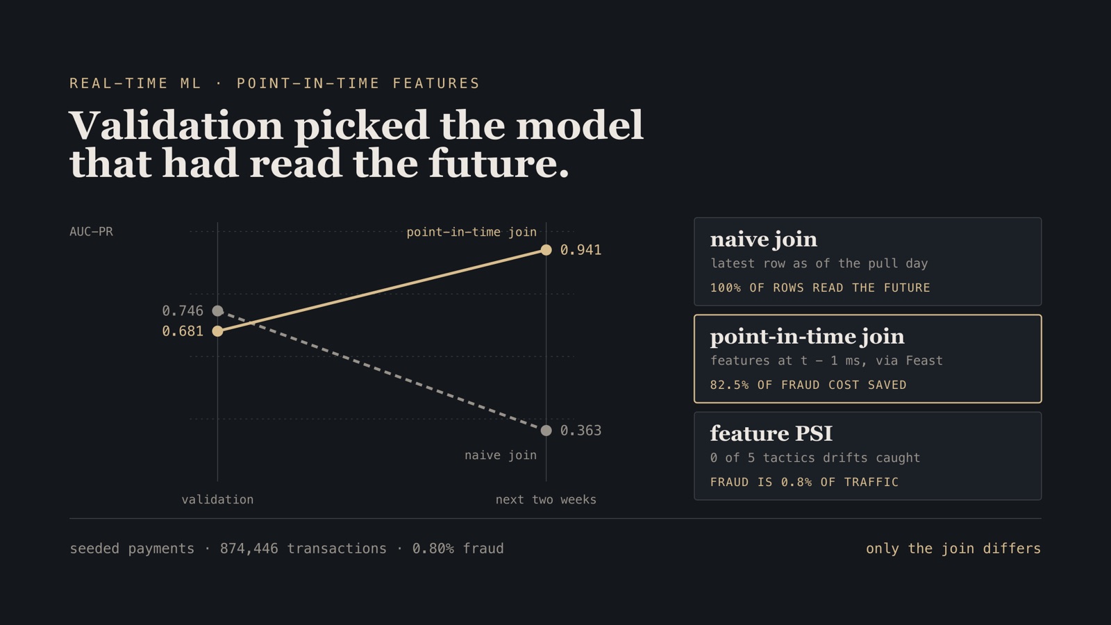
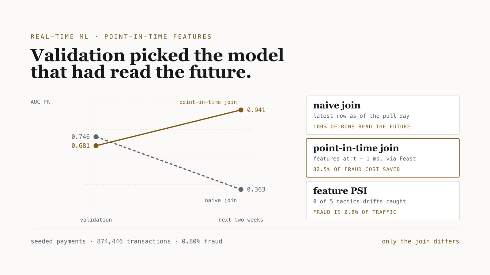
Two training sets for the same fraud model. The same transactions, the same labels, the same LightGBM hyperparameters. The only difference is how the features were joined to the rows. On the validation week, the first one scored an AUC-PR of 0.746 and the second 0.681, and the first one caught 78% of the labelled fraud at 80% precision against 36% for the second. A review that compares validation numbers ships the first.
On the two weeks that followed, scored with the features the online store would actually serve, the first model’s AUC-PR was 0.363. The second’s was 0.941. The model validation preferred was worth less than half of the one it rejected, and nothing in its offline numbers said so.
Operating rule. A training row may only see what the scoring service could have seen at the moment of the decision. Check that as a timestamp comparison on every row, in a test, rather than as a review comment. And never let a validation score settle a question about the join: a validation set built by the same pipeline inherits the same leak, and it will vote for it.
This comes from realtime-ml, a real-time fraud-scoring system I built to measure the failures that usually only get avoided: leakage, training–serving skew, late labels and drift. Payments flow through Kafka into a stream processor that keeps window features in Feast’s online store; an API scores each payment with a champion model and a challenger in shadow. The data is seeded and synthetic — 874,446 payments over 90 days for a fictional retailer, 0.80% of them fraud, with card-testing bursts, account takeovers and chargebacks that arrive weeks late. That makes the absolute scores a property of the generator. The comparisons are the point: same data, same model, one thing changed. Every figure below is in the repository’s MEASUREMENTS.md.
Two joins, one difference
The window features are what you would expect for card fraud: purchases per customer in the last day, cards seen on a device in the last hour, distinct customers on a device in the last 24 hours, chargebacks on the customer in the last 90 days. Each is stored as a row per entity per event — the entity’s state after that event.
The naive pipeline builds its training set the way one is often first built. Take the feature tables as they stand on the day the data is pulled, keep each entity’s latest row, and join on the key:
def latest_as_of(table: pd.DataFrame, keys: list[str], as_of: pd.Timestamp) -> pd.DataFrame:
    t = table[table["event_timestamp"] < as_of]
    t = t.sort_values("event_timestamp").drop_duplicates(keys, keep="last")
    return t.drop(columns=["event_timestamp"])


def naive_join(rows: pd.DataFrame, tables: dict[str, pd.DataFrame], as_of: pd.Timestamp) -> pd.DataFrame:
    out = rows
    for name, keys in (
        ("customer_velocity", ["customer_id"]),
        ("device_velocity", ["device_id"]),
        ("customer_device", ["customer_id", "device_id"]),
        ("customer_profile", ["customer_id"]),
    ):
        out = out.merge(latest_as_of(tables[name], keys, as_of), on=keys, how="left")
    return out
Nothing in it looks wrong. It filters to rows before the cut-off, which reads like a leakage guard. But the cut-off is the day the data was pulled, not the moment each transaction happened, so nearly every training row is joined to the entity’s state at the end of the window — after the transaction, after the rest of its burst, and after its chargeback if one had arrived.
The point-in-time pipeline asks Feast for each transaction’s features one millisecond before it happened:
SCORE_OFFSET = pd.Timedelta(milliseconds=1)

ent = rows[["txn_id", "customer_id", "device_id"]].copy()
ent["event_timestamp"] = rows["ts"] - SCORE_OFFSET
feats = store.get_historical_features(entity_df=ent, features=FEATURE_REFS).to_df()
The millisecond matters. A stored row is the entity’s state after an event, aggregating everything in its window up to and including that event. Scoring a transaction with the row stamped at its own time would include the transaction in its own features. Online that cannot happen — the payment is authorised before its event reaches the stream — so offline has to ask for the state after the previous event. The repository records that as a decision, along with the reason feature views carry no TTL: Feast applies a view’s TTL in historical retrieval but not on Redis reads, so a TTL would expire features offline that are still served online.
What the naive model learned instead
| Features | Join | Validation AUC-PR (labels known on the training day) | Validation recall at 80% precision | Next two weeks: AUC-PR | Next two weeks: cost saved |
|---|---|---|---|---|---|
| customer + device | naive | 0.746 | 0.779 | 0.363 | 35.0% |
| customer + device | point-in-time | 0.681 | 0.362 | 0.941 | 82.5% |
| customer only | naive | 0.551 | 0.277 | 0.180 | 20.2% |
| customer only | point-in-time | 0.412 | 0.031 | 0.613 | 66.5% |
“Cost saved” uses the repository’s cost model: every flag costs a $5 review, every missed fraud costs its amount, measured against approving everything. The pattern holds with both feature sets. The naive join wins validation and loses the future by a wide margin.
The feature importances say why. The naive model’s top features by gain were dev_txn_count_1h at 41%, cd_txn_count_30d at 21% and cust_chargebacks_90d at 17%. The first is the rest of the card-testing burst: a device that tries, say, 25 stolen cards in 40 minutes ends its burst with a one-hour count of 25, and the naive join hands that end-of-burst count to every attempt in it, including the first. Online, the first attempt in a burst sees a count near zero. The model learned a signal that only exists in hindsight.
The third is worse. cust_chargebacks_90d as of the pull day counts the chargeback for the transaction being labelled, whenever that chargeback has already arrived. The feature is partly the label.
The point-in-time model’s top features were cd_txn_count_30d at 32% and dev_distinct_customers_24h at 30%: how often this card has been seen on this device, and how many different customers one device has served in a day. Both exist at the moment of the decision, online and offline alike.
Why validation could not see it
A leak this large should be obvious, and in the textbook version it is: the leaky model posts an implausible score and someone gets suspicious. Here the leaky model posted a plausible score — 0.746 is not a number that makes anyone stop — and it beat the honest one. Two things combined to produce that.
First, the validation week was built by the same join. Its rows carried the same end-of-window features, so the leak was present on both sides of the evaluation and validation measured how well the model exploited it.
Second, the labels. A fraud only becomes a label when its chargeback arrives, after a delay with a median of seven days and a tail past a month, and 15% are never reported at all. On the training day, the validation week’s labels are the chargebacks received so far — the same chargebacks the naive model’s cust_chargebacks_90d feature was counting. Scored against the labels you have, a feature that reads those labels looks excellent.
The simulation can do something no production system can: score validation against the true labels. When it does, the ranking reverses before any future data is involved. The point-in-time model scored 0.937, the naive one 0.852. The naive model’s lead existed only against the labels a real team would be using to choose between the two.
That is the part I would carry into any model review. Leakage is usually described as a model that looks too good. The version that ships is a model that looks slightly better, against an evaluation that shares its blind spot.
The audit is one comparison per row
The good news is that this failure is cheap to detect with certainty, and it does not need a model at all. Every feature row carries the timestamp of the entity’s last event. A training row whose feature timestamp is later than the transaction has read the future:
# The shape of the check: no feature row may be newer than the event it describes.
txn_epoch = (train["ts"] - pd.Timestamp("1970-01-01", tz="UTC")).dt.total_seconds()
read_future = (train["cust_last_txn_epoch"] > txn_epoch).mean()
assert read_future == 0, f"{read_future:.0%} of training rows read the future"
In this run, 100% of the naive training rows took their customer features from a row stamped after the transaction, and 98% their device features. A point-in-time join cannot produce a single such row. The repository’s tests assert both directions: that the naive join reads the future on a small seeded dataset, and that the point-in-time features come from before the transaction. A third test checks Feast’s historical retrieval against pandas.merge_asof on the same rows, so the point-in-time join is itself verified rather than trusted.
A check like that belongs in CI beside the training code, not in a notebook someone runs when a model disappoints. It costs one comparison per row and gives a yes-or-no answer. A validation metric gives neither.
The same mistake, made with labels
The join is not the only place a fraud pipeline reads time wrongly. The labels have the same problem in the other direction: they are incomplete for recent rows, and a model trained on them without care learns that recent fraud is rare.
| Training rows | Rows | Validation AUC-PR as measured | Next two weeks: AUC-PR | Recall at its threshold | Cost saved |
|---|---|---|---|---|---|
| Everything up to the training day, labels known that day | 407,737 | 0.158 | 0.930 | 0.812 | 70.7% |
| Rows matured 14 days (the default) | 281,430 | 0.681 | 0.941 | 0.954 | 82.5% |
| Rows matured 30 days | 126,348 | 0.728 | 0.937 | 0.961 | 81.4% |
| Everything, true labels (simulation only) | 407,737 | 0.958 | 0.957 | 0.959 | 84.0% |
Training on everything with the labels known on the day barely hurt the ranking — AUC-PR 0.930 against 0.941. It ruined the threshold. Most of the validation week’s frauds were not yet labelled, so its measured AUC-PR was 0.158, and the cost-optimal threshold chosen on it flagged too little: recall fell to 0.81 and 11.8 points of cost saving were lost against the default. Waiting 30 days instead of 14 threw away 55% of the rows and gained nothing. Instant, perfect labels — the ceiling no real system reaches — were worth 1.5 points over the 14-day default.
The numbers you can see lag the truth the same way. For one day of traffic, a week later only 52% of its frauds were known; a month later, 87%; 11% never would be. Any dashboard showing recall on recent days is showing recall on the frauds reported so far: for that day, 0.865 a week later against a true recall of 0.930.
The drift monitor that never fired
The last measurement is the one that disappointed me most, and it is the same lesson from the other side of deployment. Ten seeded datasets: five where, from day 70, fraudsters slow down and stay closer to normal — card testing spread over hours instead of minutes, takeovers mostly from the victim’s home country — and every price rises 15%, and five with no drift at all. The drift cost the model 3 to 9 points of recall. Each monitor was replayed every six hours over the trailing day; a false alarm is an alert in a window with no drift in it, 650 such windows in all.
| Monitor | Drifts detected | Median time to detect | False alarms, of 650 clean windows |
|---|---|---|---|
| Feature PSI > 0.2, all features | 4 of 5 | 414 h | 50 (7.7%) |
| Feature PSI > 0.2, calendar-trending features excluded | 0 of 5 | — | 0 |
| Score PSI > 0.1 | 0 of 5 | — | 0 |
| Flag rate, |z| > 4 | 5 of 5 | 48 h | 112 (17.2%) |
| Flag rate, |z| > 8 | 2 of 5 | 84 h | 3 (0.5%) |
| Recall on arrived chargebacks down 0.10 | 3 of 5 | 300 h | 6 (0.9%) |
The four “detections” by feature PSI were not detections. All four came from cust_chargebacks_90d, which grows with the calendar as chargebacks accumulate, and it raised the same alarm in the runs with no drift. With the two calendar-trending features excluded, the largest feature PSI after onset was 0.05. The 15% price rise moved the amount feature by 0.03 to 0.04. Score PSI never passed 0.014.
The reason is arithmetic, not tuning. Fraud is 0.8% of traffic. When the fraudsters change tactics, 99.2% of the population is unchanged, and a statistic that compares populations sees almost nothing. The textbook recipe — PSI per feature against the training distribution, alert above 0.2 — is built for shifts in the whole population. A model’s failure on a rare class is not one.
What does carry signal, and what each costs:
- Recall on the chargebacks that have arrived is the only monitor that tracks the damage directly. It is about two weeks late, because the labels are, and one of its three detections was an alarm already raised before the drift began.
- The flag rate is the fastest label-free signal, and at |z| > 4 it is noise. Fraud arrives in bursts, the binomial variance is too small for that, and drift-free runs reached z = 11. At |z| > 8 it is quiet and missed three drifts in five.
- Hour-matched feature PSI is still worth running, for a different job. On the live stack, a 50% price rise fired the alert 49 seconds after the first drifted payment, and not on the day before. It catches broken inputs and pricing changes. It does not catch fraudsters adapting.
None of these caught the tactics drift both quickly and quietly, and the repository reports that as a limit instead of tuning a threshold until a chart looks good. The next thing to measure is monitoring the slice the model flags rather than all traffic — the decisions, not the population.
Boundary. The data is a seeded simulation of payments, not real fraud, and the generator’s patterns are simpler than real adversaries. Every absolute score — the 0.941 included — describes the generator. What transfers is the direction and the mechanism of each comparison: a join that reads the end of the window, a label set that is incomplete for recent rows, a population statistic watching a 0.8% class. The live stack runs every service as a container on one 8-CPU VM, so its latency and lag figures contain no network hops.
What I check before trusting a real-time model
- Every training row’s feature timestamps are earlier than its event, asserted in a test that fails the build, not inspected by eye.
- The point-in-time join is itself checked against an independent as-of join on the same rows.
- Validation features come from the point-in-time path that mirrors serving, and any comparison between two training pipelines is made on matured labels, not the labels known on the day.
- Training rows are old enough for their labels to have mostly arrived, and the threshold is chosen on a window whose labels are mature.
- Feature parity between the batch and stream implementations is compared feature by feature, because a model-level check passes defects in features the current model barely uses.
- Drift monitors are tested against a drift that hurts the model and against no drift at all, and their false-alarm rate is published next to their detection rate.
Frequently asked questions
What is a point-in-time join, and how does a naive join leak?
A point-in-time join gives each training row the feature values as they stood just before the event. In realtime-ml, Feast’s historical retrieval is asked for features at the transaction time minus 1 ms. The naive join took each entity’s latest row as of the day the data was pulled, so 100% of training rows took customer features, and 98% device features, from after the transaction.
Why did the leaky model score higher on validation?
The validation rows were built by the same join and scored with the chargebacks known on the training day. One of the naive model’s strongest features counts chargebacks, including the transaction’s own, so feature and label partly come from the same records. Scored against true labels, which only a simulation has, the ranking reversed: 0.937 for the point-in-time model, 0.852 for the naive one.
Why did PSI miss the fraud drift?
Fraud was 0.8% of traffic. When fraudsters slowed down and stayed closer to normal, recall fell 3 to 9 points, but the largest feature PSI after onset, with calendar-trending features excluded, was 0.05, and score PSI never passed 0.014. The population did not move enough for a population statistic to notice.
What should a fraud drift monitor watch instead?
Recall on the chargebacks that have arrived tracks the real damage but caught 3 of 5 drifts about 300 hours late. The flag rate is the fastest label-free signal, but at |z| > 4 it fired on 17.2% of drift-free windows and at |z| > 8 it missed 3 of 5. None caught the drift both quickly and quietly; watching the flagged slice instead of all traffic is the next thing to measure.
The system behind these numbers — Kafka, the stream processor, Feast, the shadow challenger and the paired promotion gate built on evalproof — is described in the realtime-ml case study, and the code, seeds and commands are in the repository. A related problem with labels and trends, where counting a classifier’s output flattens what it measures, is in The classifier was 95% accurate. The trend it counted was a third too flat.