On this page
A retrieval query for a RAG system almost always has a filter on it. The user may only see their own tenant’s documents, or this year’s, or one product’s. In Postgres it reads like any other query:
SELECT id FROM docs
WHERE tenant_id = $2
ORDER BY embedding <#> $1
LIMIT 10;
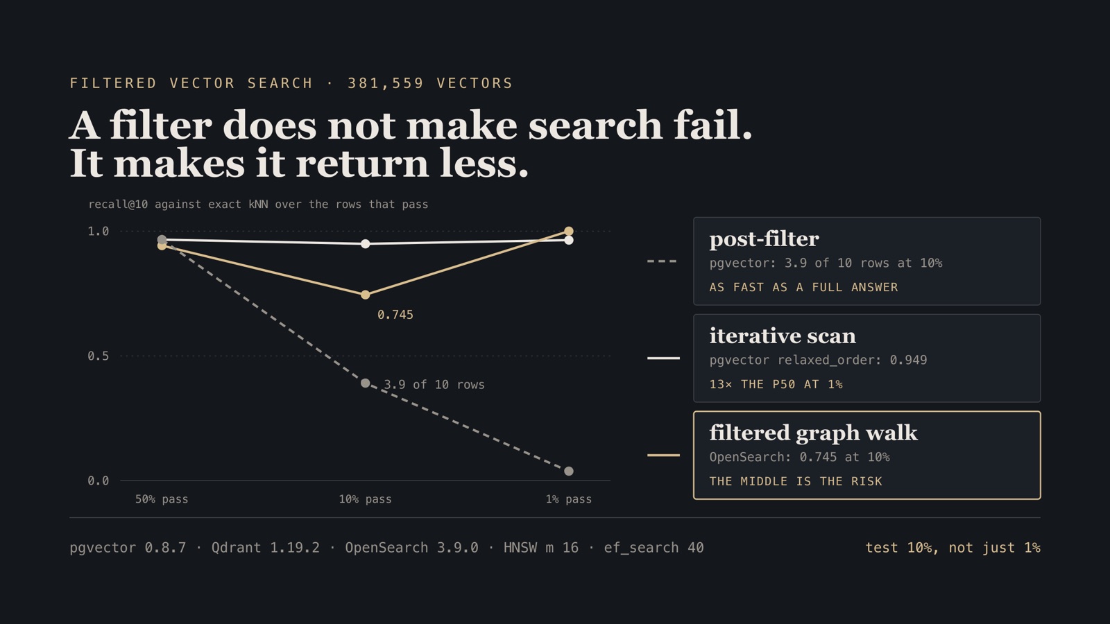
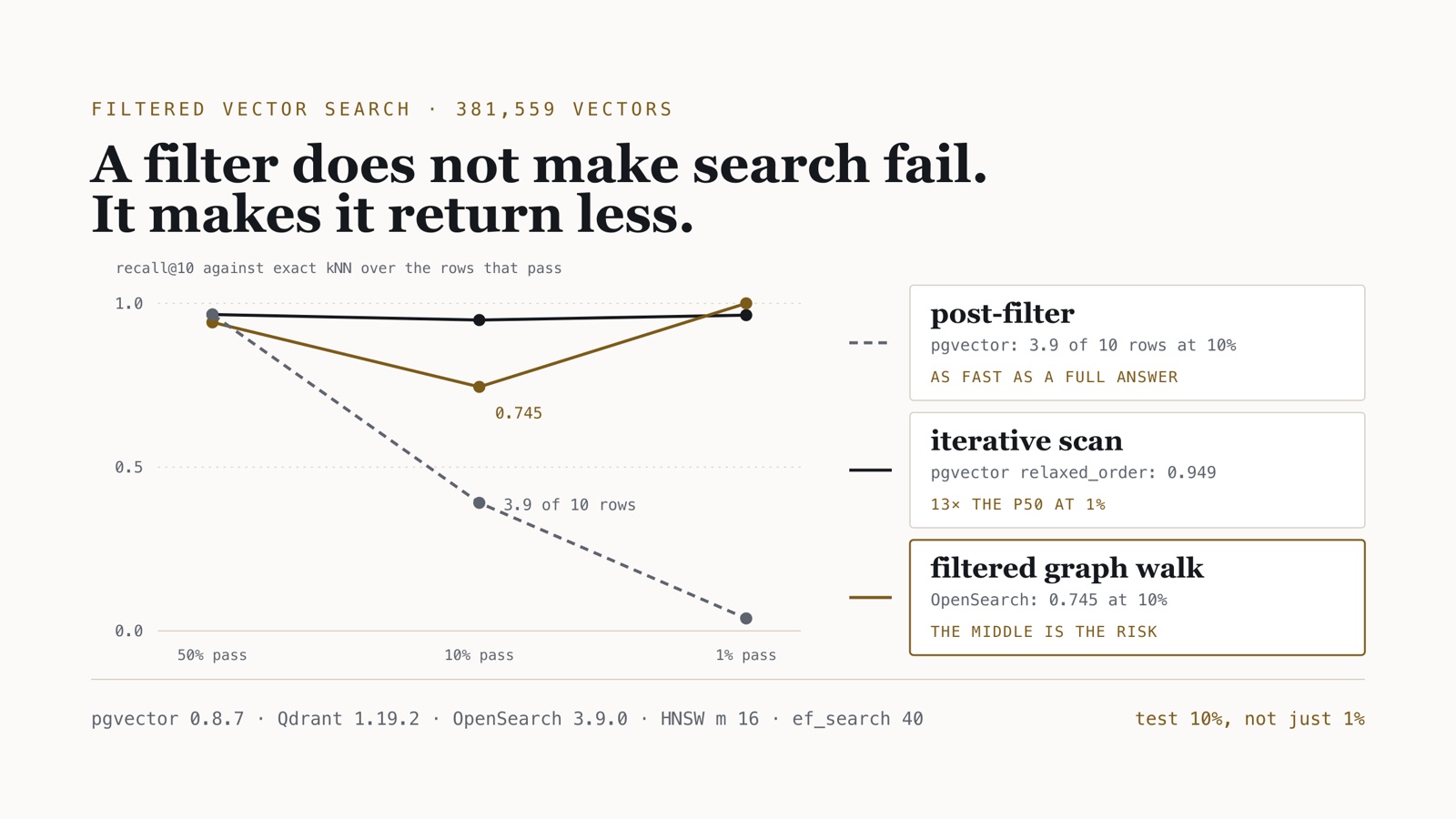
On a table with an HNSW index this comes back in well under a millisecond. On my benchmark, when the filter kept a tenth of the rows, it came back with four rows instead of ten. When it kept one row in a hundred, it came back with fewer than one on average. There was no error, no warning and no slow query to notice: the short answers took exactly as long as full ones. A language model downstream would have answered from whatever arrived.
Operating rule. Never measure a vector index only unfiltered. Sweep the filter’s selectivity — half the rows, a tenth, a hundredth — compare each result against exact search over the rows that pass, and count how many rows came back. The two extremes are the cases engines handle; the middle is where they quietly lose part of the answer.
The numbers come from retrieval-bench, which loads one set of embeddings into pgvector, Qdrant and OpenSearch and measures them under identical limits. The filtered runs were one section of it. They are the section that changed what I would ship.
The rig
The corpus is args.me, the document collection of Touché 2020: 382,545 arguments, minus 986 near-duplicates of the query set, leaving 381,559 vectors of 384 dimensions from bge-small-en-v1.5, embedded once and loaded unchanged into every engine. The queries are the first 1,000 from ArguAna. args.me, the Touché 2020 topics and judgements, and ArguAna are all released under CC BY 4.0, and the repository’s NOTICE credits each at its original source; no corpus text is committed.
Three engines, pinned: PostgreSQL 18 with pgvector 0.8.7, Qdrant 1.19.2 and OpenSearch 3.9.0 with its Faiss HNSW. Each runs in its own container, limited to 4 CPUs and 5 GiB, and only the engine under test runs while anything is timed. HNSW is built with m = 16 and ef_construction = 100 everywhere, and every engine is queried at ef_search = 40 — the smallest swept value at which all three reached recall@10 of 0.95 unfiltered, and also pgvector’s default.
The filter is deliberately artificial. Each document carries a bucket from 0 to 99, taken from a hash of its id, so bucket < 50, < 10 and < 1 keep 50%, 10% and 1% of rows. Because it is a hash, it has nothing to do with content — the hardest case for a graph index and the cleanest test of one. Ground truth is brute-force inner product in numpy over exactly the rows that pass, so recall@10 asks one question: of the ten true nearest neighbours that satisfy the filter, how many came back?
Timing is client-observed, after a full warm-up pass, as the median of five passes interleaved across the sweep. The method and every table are in MEASUREMENTS.md.
Post-filtering returns what the arithmetic allows
| Engine and strategy | 50%: recall · rows · p50 | 10%: recall · rows · p50 | 1%: recall · rows · p50 |
|---|---|---|---|
| pgvector HNSW, iterative scan off | 0.966 · 10.0 · 0.69 ms | 0.391 · 3.91 · 0.63 ms | 0.038 · 0.38 · 0.65 ms |
| OpenSearch, filter beside the knn clause | 0.511 · 5.13 · 0.82 ms | 0.099 · 0.98 · 0.70 ms | 0.010 · 0.10 · 0.74 ms |
pgvector HNSW, relaxed_order |
0.966 · 10.0 · 0.68 ms | 0.949 · 10.0 · 1.26 ms | 0.964 · 10.0 · 8.77 ms |
pgvector HNSW, strict_order |
0.966 · 10.0 · 0.66 ms | 0.908 · 10.0 · 1.45 ms | 0.896 · 10.0 · 9.22 ms |
| Qdrant, payload index | 0.936 · 10.0 · 0.72 ms | 0.925 · 10.0 · 0.64 ms | 1.000 · 10.0 · 0.82 ms |
| OpenSearch, efficient filter | 0.942 · 10.0 · 0.84 ms | 0.745 · 10.0 · 0.81 ms | 1.000 · 10.0 · 1.01 ms |
The first two rows are post-filters, and they do exactly what the arithmetic says. With iterative scans off, pgvector’s HNSW index scan hands Postgres ef_search candidates — forty — and the WHERE clause runs on those. A tenth of forty is four: the measured mean was 3.91. A hundredth of forty is 0.4: the measured mean was 0.38. Every filtered query used the vector index; the plan is recorded in the results file, and there is no B-tree on bucket for the planner to prefer.
OpenSearch shows the same shape one step earlier. With the filter placed beside the knn clause in a bool query, k-NN returns its top ten and the filter runs on those: 5.1, 1.0 and 0.1 rows at the three selectivities.
The column that matters most is latency. A post-filtered query that returns 0.38 rows took 0.65 ms; an unfiltered one took 0.66. A dashboard of p95s would show a healthy retriever. An error-rate panel would show nothing at all, because nothing failed. The only signals are the number of rows that came back, which most retrieval code never logs, and a comparison against exact search, which nobody runs in production.
Three answers to a selective filter
The other four rows are the engines doing something about it, and they do three different things.
Keep walking. pgvector 0.8 added iterative index scans. With hnsw.iterative_scan = relaxed_order, when too few candidates pass the filter the scan continues through the graph until enough do, up to hnsw.max_scan_tuples. It brought recall back to 0.949 at 10% and 0.964 at 1%, and it charged for it: 1.9× the unfiltered median at 10%, 13× at 1%, where it has to walk past roughly a hundred rejected rows for every one it keeps. strict_order, which keeps results in exact distance order, cost more and recalled less (0.908 and 0.896), so relaxed_order is the setting I would use. The fix is two settings and the same query:
SET hnsw.ef_search = 40;
SET hnsw.iterative_scan = relaxed_order;  -- pgvector 0.8+
SELECT id FROM docs
WHERE bucket < 10
ORDER BY embedding <#> $1
LIMIT 10;
Walk a graph that knows about the filter. Qdrant had its payload index on bucket before the graph was built, which lets it add extra links for indexed payload values so the graph stays navigable when most nodes are excluded. OpenSearch’s efficient filter — the filter inside the knn clause rather than beside it — runs a filtered HNSW traversal per segment. Both return ten rows at every selectivity, because the filter is part of the search rather than applied to its output:
{
  "size": 10,
  "query": {
    "knn": {
      "vec": {
        "vector": [0.0367, -0.0284, 0.0630],
        "k": 10,
        "filter": { "range": { "bucket": { "lt": 10 } } }
      }
    }
  }
}
(The vector is shortened here; the real one has 384 values.)
Give up on the graph. At 1%, about 3,800 rows pass. Scoring all of them exactly is cheap, and both Qdrant and OpenSearch decided so: recall 1.000, in 0.82 and 1.01 ms. That is why the most selective filter turned out to be the easy case. It is also the case most teams test, because “a small tenant” is the obvious filter to try.
Why 10% is the risk
At 10%, about 38,000 rows pass. That is too many for either engine to fall back to exact search, so both walk the graph — a graph in which nine of every ten nodes must be stepped through but cannot be returned. Qdrant held 0.925, against 0.974 unfiltered at the same ef_search. OpenSearch’s efficient filter fell to 0.745: it returned a full ten rows, and about a quarter of them were not among the ten nearest that pass.
That number is outside the noise of the rig. HNSW builds are multi-threaded and vary: three OpenSearch builds gave unfiltered recall of 0.949, 0.962 and 0.965 at this setting. A drop of twenty points is not build variance. I have not traced inside Faiss why the filtered walk loses that much at this selectivity, and the repository says so. What I can say is where it sits: between the selectivity at which the engine trusts its graph and the one at which it stops trusting it.
This failure is worse than the post-filter’s in one respect. A post-filter’s short answer is visible in a row count. A filtered graph walk that returns ten slightly wrong rows is visible only against exact search. Nothing in the response distinguishes a 0.745 answer from a 1.000 one.
Two qualifications keep this honest. Recall here is measured against exact nearest neighbours, not human relevance judgements, so a missed neighbour is a retrieval error, not necessarily a wrong answer; the benchmark does not score filtered results for relevance. And ef_search is a lever: a larger value buys back recall at the cost of latency, and the sweep in MEASUREMENTS.md shows how much each engine charges for it unfiltered. Neither changes the operating point most systems run at, which is whatever recall the unfiltered benchmark said was enough.
What the filter changes about choosing an engine
Unfiltered, the three engines were hard to tell apart. Given the same vectors, their retrieval quality was within 0.0015 nDCG@10 of exact search on SciFact, ArguAna and Touché 2020, and at recall@10 ≈ 0.97 their median latencies were 0.66, 0.68 and 0.79 ms on round-trip floors of 0.15 to 0.28 ms. A benchmark that stops there concludes the choice does not matter.
The filtered runs say the choice is about behaviour under a filter, and that each engine needs something different to get it right:
- pgvector needs
relaxed_orderturned on, and a latency budget for the very selective filters where it walks the longest. - OpenSearch needs the filter inside the
knnclause, never beside it, and a recall check at the middle selectivities its exact fallback does not cover. - Qdrant needs its payload index created before the graph is built, which is when the extra links are added.
IVFFlat, for completeness, did not collapse: at 16 probes it scans about 15,000 rows per query, so even 1% leaves around 150 candidates. Its recall at 1% (0.840) was lost to the lists it did not probe, and at 3.7 to 4.4 ms per query it was the slowest option throughout; unfiltered, it already needed 5.7× pgvector HNSW’s latency for the same recall.
Boundary. One synthetic filter, uncorrelated with content. Real tenant and date filters correlate with what a document says, which can help a graph walk (the passing rows sit near each other) or hurt it (the query lands far from them); this run measures neither. Everything fits in memory, on one node per engine, with shared index parameters rather than tuned ones, and OpenSearch force-merged to one segment. The engines run in Docker’s VM on the same host as the client — an Apple M5 with 10 cores and 24 GiB — so there is no network between application and database, other applications shared the machine, and a network filter on the host sees the loopback traffic. Interleaved passes and medians blunt that; they do not remove it. Every figure is in the repository’s MEASUREMENTS.md, drawn from the JSON results it commits.
What I check before trusting a filtered retriever
- Recall@10 against exact search over the passing rows, at 50%, 10% and 1% selectivity, at the
ef_searchthe service actually runs. - Mean rows returned at each selectivity; anything below
kwith no error is a post-filter. - The query plan or request shape: pgvector with
iterative_scanset, OpenSearch with the filter insideknn, Qdrant with the payload index built before the graph. - p50 and p95 at the most selective filter, where an iterative scan pays the most.
- A rows-returned counter in production retrieval logs, because it is the one failure signal that costs nothing.
- A periodic sample of production queries re-run as exact search with their filters, because a filtered graph walk’s misses show up nowhere else.
Frequently asked questions
Why does a pgvector query with a WHERE clause return fewer rows than its LIMIT?
Without an iterative scan, the HNSW index produces ef_search candidates, 40 by default, and the WHERE clause runs on those. With a filter that keeps 10% of rows, about four of the forty pass. In this benchmark pgvector returned 3.9 rows of 10 at 10% and 0.38 at 1%, as fast as a full answer and with no error or warning.
What is the difference between relaxed_order and strict_order in pgvector?
Both are iterative index scans, added in pgvector 0.8: when too few candidates pass the filter, the scan keeps walking the graph, up to hnsw.max_scan_tuples. strict_order keeps results in exact distance order; relaxed_order lets them come back slightly out of order. Here relaxed_order recalled more (0.949 against 0.908 at 10%) and cost less.
Do Qdrant and OpenSearch have the same problem?
Not in the same form when the filter is part of the vector query. Both switched to exact search at 1% and returned perfect results in about a millisecond. Their weak spot was 10%: Qdrant recalled 0.925 and OpenSearch’s efficient filter 0.745, both while returning ten rows. A filter placed beside OpenSearch’s knn clause in a bool query is a post-filter and collapses like pgvector’s.
How should a filtered retriever be tested?
Sweep several selectivities, not just none and one very selective filter, and compare each against exact nearest neighbours over the rows that pass. Record how many rows came back as well as recall: a post-filter’s short answers show in the row count, and a filtered graph walk’s misses only show against exact search.
The whole benchmark — quality, latency, build cost, concurrency and writes under load — is written up as a case study in retrieval-bench. The retrieval pipeline it was built to inform is in the lakehouse RAG lab. More on RAG and Postgres.